Finance tool
cb-terminal
Local terminal built for convertible bond analysis.
The problem
Convertible bond (CB) trading still requires a lot of manual oversight: most trades are executed in chatrooms, and price quotes are not standardized across brokers. As every bond has different terms and features, CBs are inherently complex instruments. Trading is further complicated because execution is sometimes on a “hedged basis” (e.g., fixing the pricing relationship between the bond and the underlying stock).
Due to these factors, existing financial software often lacks the ability to provide comprehensive time-series analysis, and customized tools are preferred for valuation and analytics. Therefore, the goal is to build a tool that is tailored for convertible bond analysis and supports better trading decisions.
Workflow
Inputs
Ingest & normalize
Decision outputs
The terminal
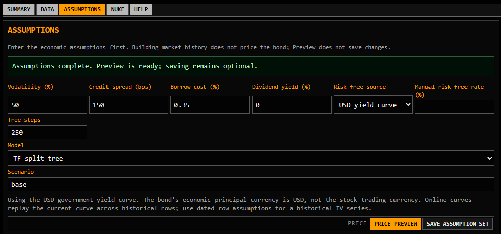
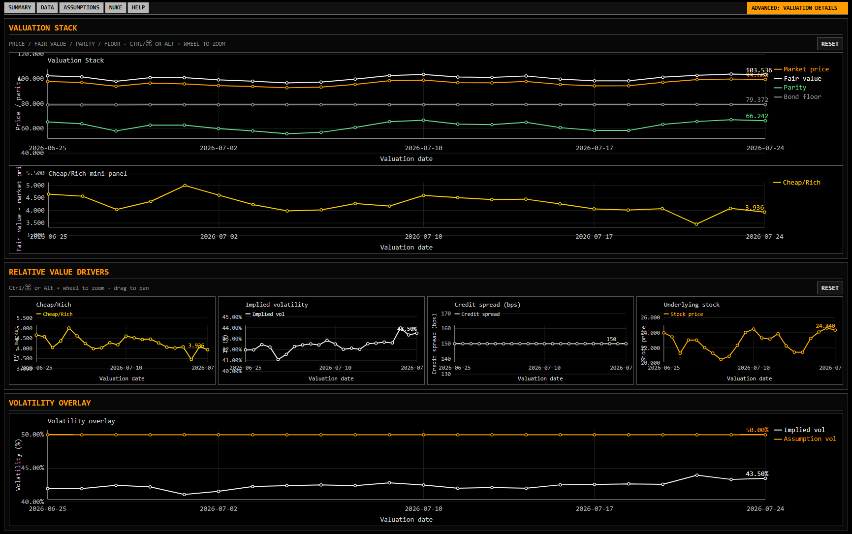
Screenshots of the assumptions and valuation output pages:
The valuation model
The production model, tf_split_tree:v2, is a one-factor, constant-parameter Tsiveriotis–Fernandes (TF) lattice. It combines a recombining Cox–Ross–Rubinstein stock tree with a split valuation: conversion-contingent value is discounted at the risk-free rate, while cash-only value is discounted at the risk-free rate plus a credit spread. [1] [2]
1. Build the stock tree
Under the risk-neutral measure, the stock follows an effective-carry process:
Where S is the underlying stock price, r is the risk-free rate, q is the dividend yield, b is the stock-borrow cost, σ is annualized volatility, dt is a small time interval, and dW is a random price shock.
For a step of length Δt, the CRR moves and risk-neutral probability are:
Where u and d are the stock-price multipliers for an up or down move, p is the risk-neutral probability of an up move, 1−p is the probability of a down move, Δt is one tree step, and e denotes exponential compounding.
2. Split equity and cash value
At each node, total CB value V is split into an equity/conversion component E and a cash-only component C. If s is the credit spread:
Where E is the conversion-linked component, C is the cash-only component, V is their combined value, s is the issuer credit spread, and the up and down subscripts refer to the two possible next-step nodes.
Conversion sets (E, C) = (kS, 0), where k is the conversion ratio. A cash put sets (E, C) = (0, P). Coupons are added at their payment nodes before the holder chooses whether to continue or convert.
3. Apply holder and issuer rights
The lattice works backward through each date, applying the holder’s floor L and the issuer’s ceiling H simultaneously. The issuer ceiling is the greater of the cash call price and the value received through forced conversion:
Where L is the value floor created by the holder’s conversion and put rights, H is the ceiling created by the issuer’s call right, and Vcontinuation is the value of holding the bond for another step.
At maturity, the bond pays the greater of cash redemption plus the final coupon and conversion value:
Where VT is the bond value at maturity, k is the number of shares received per bond, and ST is the stock price at maturity.
This backward induction models coupons, early conversion, scheduled puts, multiple call schedules, and maturity redemption in one framework. The engine also calculates parity, delta, conventional yield to maturity and yield to put, and implied volatility conditional on the selected credit spread.
Judgment & limits
- Flat inputs: rates, credit spread, volatility, dividends, and borrow cost remain constant throughout each valuation run; term structures and changing market regimes are not modeled.
- Credit-risk approximation: the TF split-discounting approach has known shortfalls. For example, TF applies a credit spread to the bond-like portion instead of modeling default directly. Therefore, recovery, the stock-price reaction to default, and the relationship between credit and equity risk are handled only implicitly, which can cause inconsistencies around calls and conversion.
- Contract details: some features ncluding call notice periods, conversion-price resets, dilution adjustments, and event-triggered puts are simplified or not yet supported.
- Cross-currency simplification: the one-factor model omits FX volatility, stock/FX correlation, and quanto effects.
- Numerical and data sensitivity: results depend on tree resolution, clean market histories, correct identifiers, currency conventions, and the selected risk-free curve.
References
-
[1]
Cox, J. C., Ross, S. A., & Rubinstein, M. (1979). “Option pricing: A simplified approach.” Journal of Financial Economics, 7(3), 229–263. DOI
-
[2]
Tsiveriotis, K., & Fernandes, C. (1998). “Valuing convertible bonds with credit risk.” The Journal of Fixed Income, 8(2), 95–102. DOI
-
[3]
Ayache, E., Forsyth, P. A., & Vetzal, K. R. (2003). “Valuation of convertible bonds with credit risk.” The Journal of Derivatives, 11(1), 9–29. DOI
-
[4]
Zabolotnyuk, Y., Jones, R., & Veld, C. (2010). “An empirical comparison of convertible bond valuation models.” Financial Management, 39(2), 675–706. DOI