Connectomics
connectome-graph-analysis
An exploratory analysis using graph-theoretic features and machine learning to test whether connectome patterns can support subject sex prediction for the SWU4 dataset.
Overview
This is an exploratory analysis project extended from a course assignment that uses graph-theoretic features and machine learning to test whether connectomic features can predict subject sex in the SWU4 dataset.
The objective is to build a classifier and obtain a classification score of 70% or higher.
The data
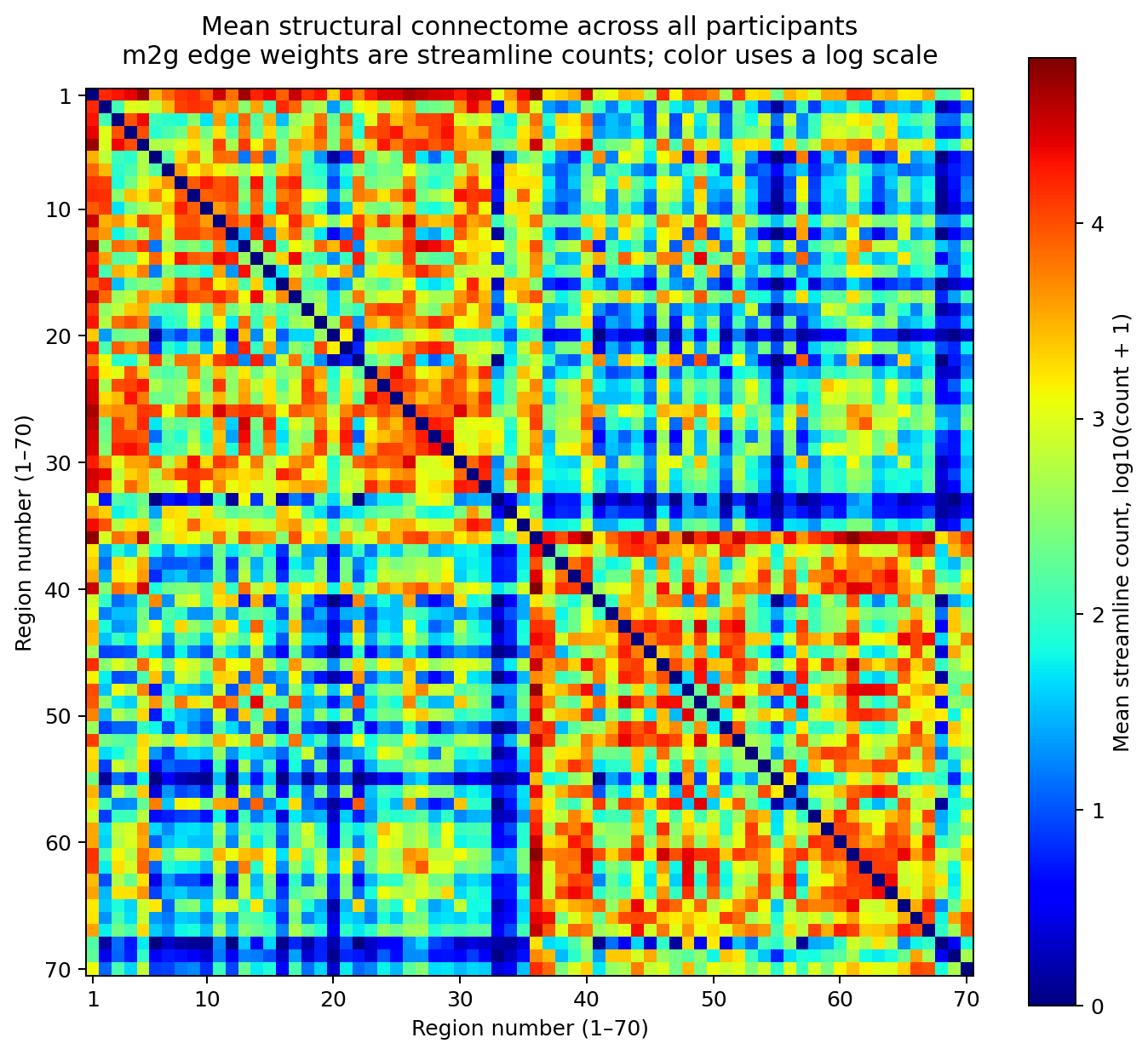
The project starts with precomputed SWU4 weighted edge lists. Each connectome file contains three columns: two nodes and a weight. The nodes are Desikan atlas brain regions, and the weight describes the estimated strength of the structural connection between them.
The matched dataset contains 207 subjects between the ages of 17 and 27: 99 with sex label 1 and 108 with label 2. Each connectome has 70 regions, so the same region-to-region connections can be compared across subjects.
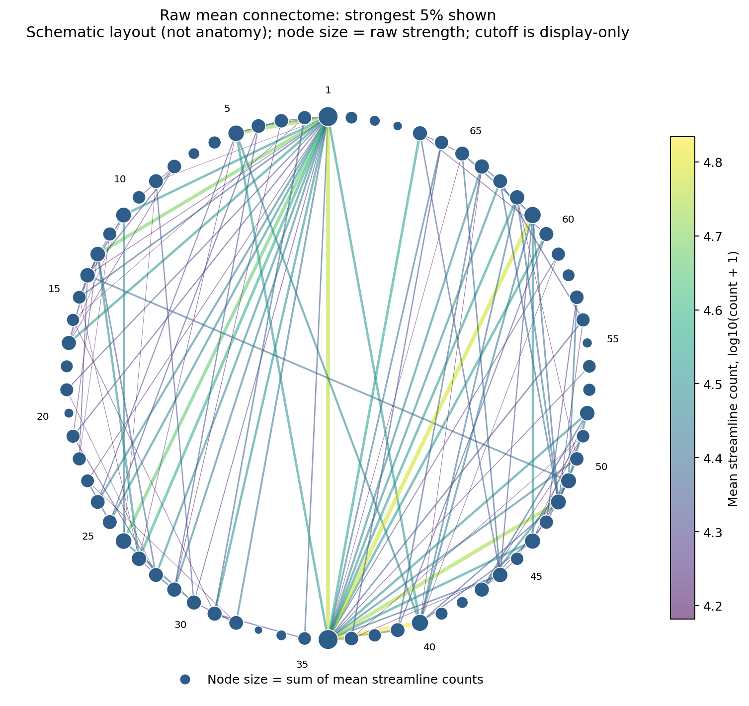
The same group-average connectome can also be represented as a network. This view below keeps only the strongest 5% of mean connections so the dominant edges remain visible.
Feature extraction
Each connectome was turned into one row of numbers. The features can be categorized into three families: graph features, topology features, and log-scaled edge weights.
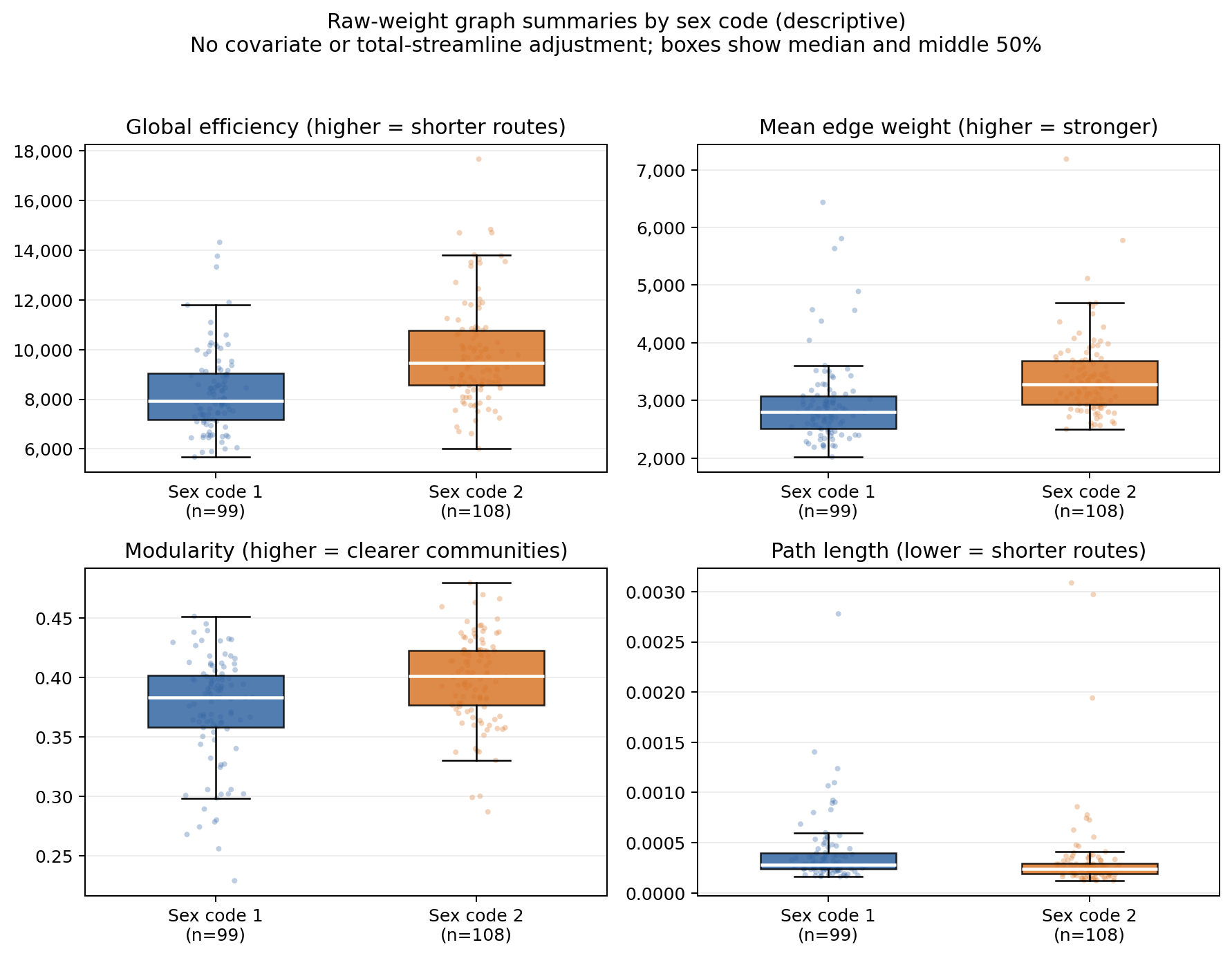
Graph features
- Global efficiency: how efficiently regions can communicate through short paths. Stronger connections are treated as shorter distances.
- Edge-weight statistics: the mean, standard deviation, median, and 25th and 75th percentiles of connection strength.
- Modularity: how strongly the graph separates into communities that are more connected internally than they are to the rest of the network.
- Characteristic path length: the average weighted shortest-path distance between regions.
- Node strength: the total connection weight attached to each region.
Topology features
- Weighted clustering coefficient: whether a region's neighbors are also strongly connected to one another.
- Betweenness centrality: how often a region lies on the shortest paths between other regions.
- Closeness centrality: how close a region is to the rest of the network by weighted shortest paths.
- Participation coefficient: whether a region spreads its connections across several communities instead of concentrating them within one.
Edge-weight features
While the graph and topology features summarize the network, the edge-weight features are more detailed and allow the model to capture the weight of every individual region-to-region connection.
Each weight was transformed with log10(weight + 1) so the large weights do not overwhelm the smaller connections.
Model and validation
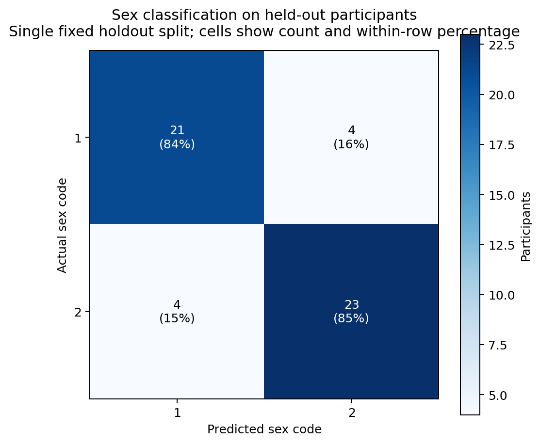
The classifier is a random forest with 300 decision trees. The data was split into a 75% training set and a 25% holdout set, and the label proportions are similar in both. The performance is also validated using shuffled, stratified five-fold cross-validation.
Results
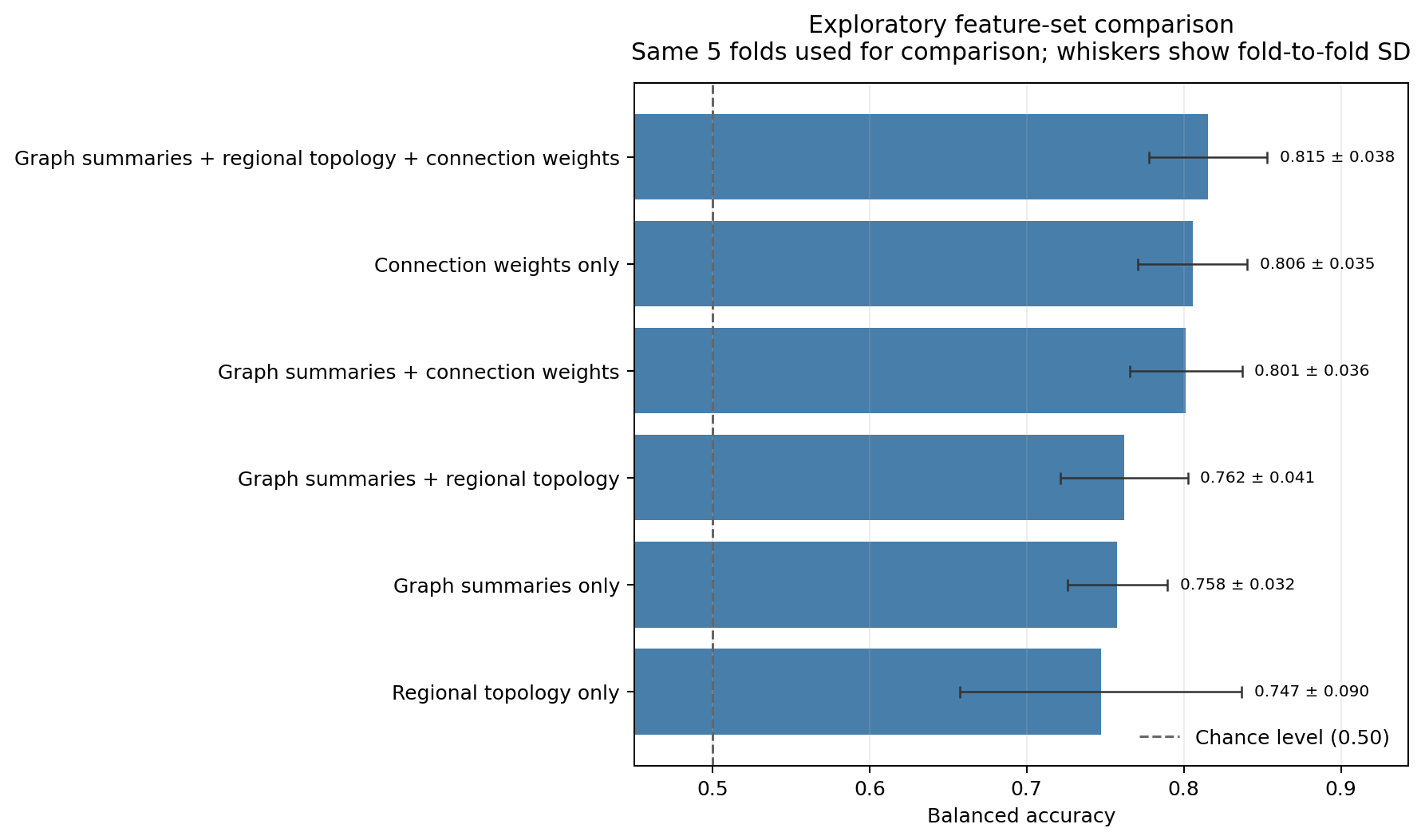
The full feature set performed best: 81.5% ± 3.8% balanced accuracy across five-fold cross-validation and 84.6% on the holdout set.
- Graph + topology + log edge weights: 81.5% cross-validated balanced accuracy
- Log edge weights only: 80.6%
- Graph features only: 75.8%
- Topology features only: 74.7%
Discussion
This project demonstrates how structural connectomes can be represented as graphs, analyzed using graph-theoretic features, and used for machine-learning classification. However, this analysis is only exploratory because it includes a relatively small dataset. The results are limited by the quality and information available in the data. Overfitting is a key concern, as there are more features than subjects. A stronger follow-up study should be tested on an independent dataset and control more carefully for other baseline differences, such as age and total streamline count.